Catenary objects: putting a wire between two points (in 3D)
Modelling a hanging physically/geometrically correct chain supported only at its endpoints.
this blog was last updated November 18, 2025
A seemingly trivial problem that is non-trivial: catenaries
Because gravitational force is so ubiquitous, we think of an objecting hanging and sagging as intuitive and – at least I for my part – trivially solved. Suppose we have two points and a line of given length, how do we model the underlying sagged rope/chain/cable? Mathematically, we call the resulting shape a catenary:
In physics and geometry, a catenary (US: /ˈkætənɛri/ KAT-ən-err-ee, UK: /kəˈtiːnəri/ kə-TEE-nər-ee) is the curve that an idealized hanging chain or cable assumes under its own weight when supported only at its ends in a uniform gravitational field
.
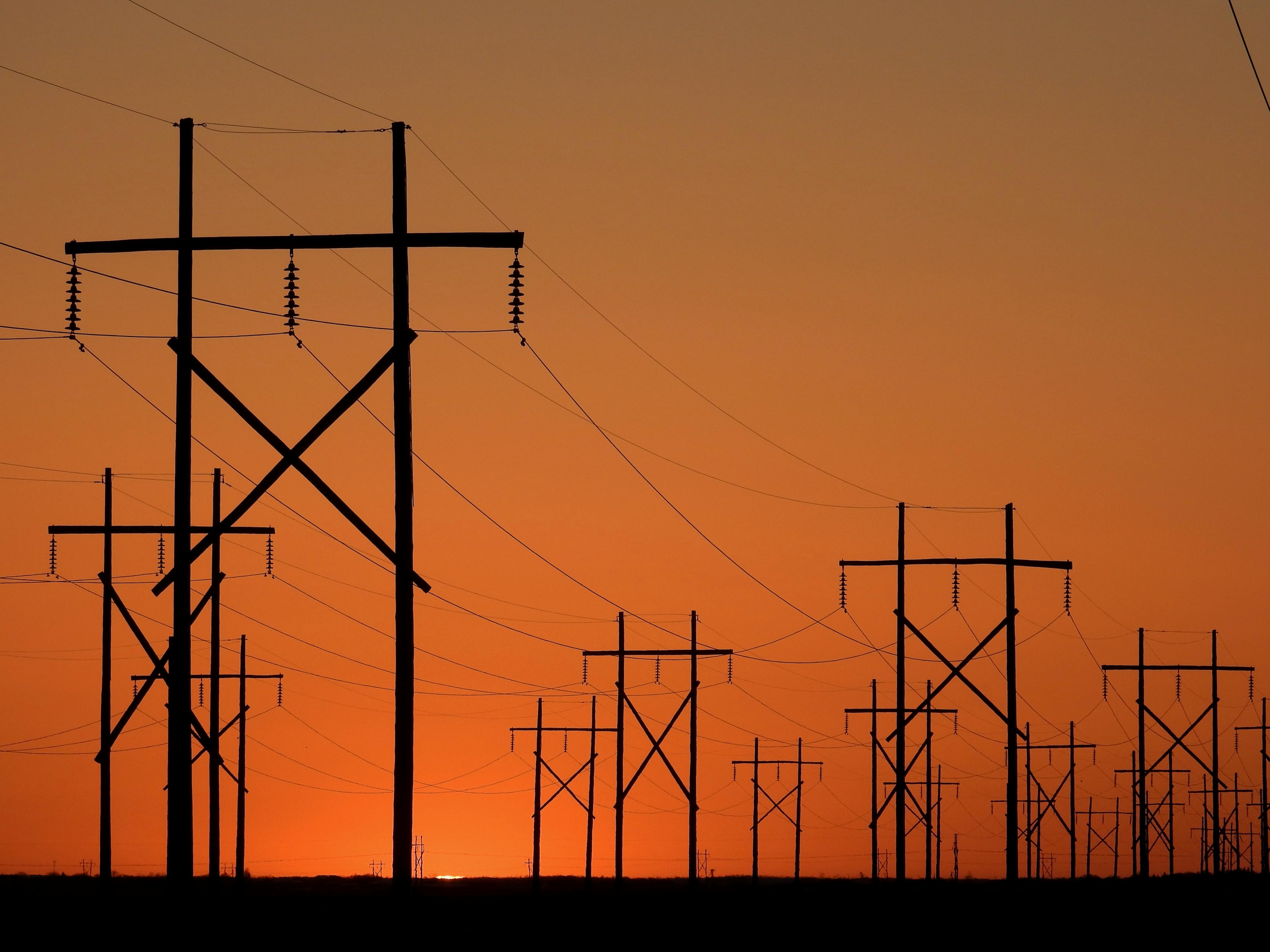
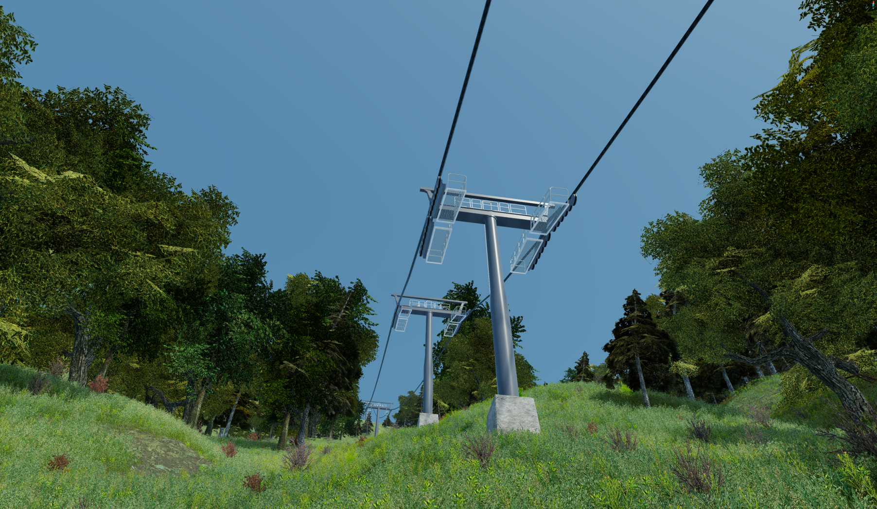
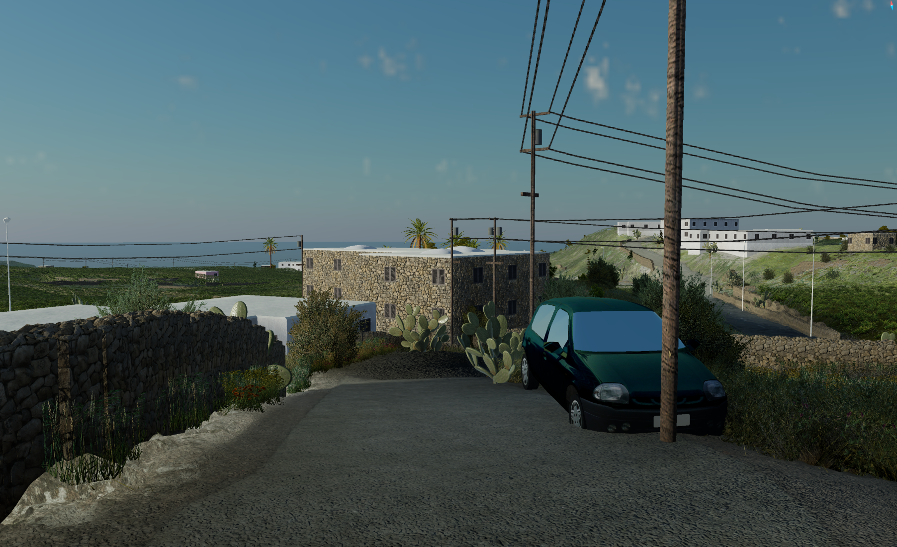
This implementation was motivated by power lines in the real world, they never form a straight line between pylons. They sag, sometimes severely: when the material of the cables heat up, they expand causing them to sag more. This reoccurring sagging behavior is applicable to many objects in real world: overhead-cables for trains, cable cars, fences, even some natural phenomena like heavy wine branches or spider webs.

In the LandscapeLab – a data driven, generic 3D landscape visualization toolkit – we abstracted this behavior for reusability as “connected” objects. In this blog we learn how to define:
- the exact length of the cable (as a factor over straight-line distance)
- arbitrary 3D positions of the two endpoints in the landscape
That combination turns out to be more subtle than just “interpolate some points” or “throw a quadratic at it”. This post walks through how we solved it numerically and how we map the solution back into 3D space.
Why a simple interpolation isn’t enough
If we only cared about a nice looking curve between two points $P_1$ and $P_2$, we could use a Bézier curve, or a spline. But all of these suffer from one big issue: You don’t control the physical length of the wire.
In reality, a cable has a fixed length. If you move the poles further apart or change their relative height, the curve must adapt so that:
- it still connects $P_1$ and $P_2$ exactly
- the arc length of the curve is a given value $L$ (e.g. straight-line distance $\times$ some factor)
That constraint leads you directly into the catenary.
The catenary problem
According to a post by Marty Cohen on StackExchange
We want to find parameters $a, b, c$ such that:
- The curve passes through both endpoints:
- The arc length between the endpoints equals a given total length $L$:
Solving for the parameters numerically
Following the derivation in Cohen’s post
, where:
\[dx = x_2 - x_1,\] \[\hat{x} = (x_1 + x_2) / 2,\] \[dy = y_2 - y_1,\] \[r = \sqrt{L^2 - dy^2} / dx.\]Consequently, we need to solve $r=\sinh(A)/A$ for $A$ numerically for given $r$. While a simple linear search is sufficient (i.e. increasing $A$ in small steps until $rA < \sinh(A)$), more advanced root-finding methods like Newton’s iteration may be used, we apply:
\[A_{n+1} = A_n - \frac{r A_n - \sinh(A_n)}{r - \cosh(A_n)}\], until
\[|r A_n - \sinh(A_n)| < \epsilon\]for some small $\epsilon$.
The initial value, $A_0$ for the iteration is defined as:
\[A_0 = \begin{cases} \sqrt{6(r-1)}, & \text{ if } r < 3 \\ \ln(2r)+\ln(\ln(2r)), & \text{otherwise} \end{cases}\]Solving the catenary in practice
In this section, we walk through how we implemented the above logic in GDScript for LandscapeLab, and provide a Python reference implementation for clarity.
Python
The above logic can be implemented in Python as follows:
def cosh(z): return (exp(z)+exp(-z))/2
def sinh(z): return (exp(z)-exp(-z))/2
def tanhi(z): return 0.5*log((1+z)/(1-z))

def solve_catenary(P1: np.ndarray, P2: np.ndarray, length: float) -> tuple[np.ndarray, np.ndarray]:
    dx = P2[0] - P1[0]
    dy = P2[1] - P1[1]
    xb = (P1[0] + P2[0]) / 2.0

    if length <= np.linalg.norm(P2 - P1):
        raise ValueError(
          "Catenary length must exceed straight-line distance between points"
        )
    if abs(dy / length) >= 1:
        raise ValueError(
          "Length too short for vertical separation"
        )

    r = sqrt(length**2 - dy**2) / dx
    A = sqrt(6*(r-1)) if r < 3.0 else np.log(2*r) + np.log(np.log(2*r))
    while abs(r-sinh(A)/A) > 1e-3:
        A -= (sinh(A)-r*A)/(cosh(A-r))

    a = dx / (2 * A)
    b = xb - a * tanhi(dy / length)
    c = P1[1] - a * cosh((P1[0] - b) / a)

    x_vals = np.linspace(P1[0], P2[0], 600)
    y_vals = np.array([a * cosh((x - b) / a) + c for x in x_vals])

    return x_vals, y_vals
Using this function, you can compute the catenary curve between two 2D points P1 and P2 with a specified length. In the plotly plot below, we visualize a catenary between points:
P1 = np.array([-0.2, 0.1])P2 = np.array([0.3, 0.0])
with a length between 0.0.
Porting to godot
Trivially, python and GDScript are similar enough that the above code can be ported almost 1:1. However, we have to put some additional thought:
- In a generic toolkit, having to use a length in absolute units is inconvenient. Instead, we want to specify a length factor (0.0 -> straight line, 0.1 -> 10% more longer) over the straight-line distance between the two endpoints, like:
var straight = P1_2D.distance_to(P2_2D)
var L = straight + straight * length_factor
- The endpoints are in 3D space, not 2D. We need to project them into a 2D plane, solve the catenary there, and then map the resulting curve points back into 3D.
- In a large generic world, performance matters: To avoid recomputing the same catenary multiple times (e.g. when many cables share the same geometry but are just translated in space), we want to cache previously computed curves.
Firstly, the GDScript version of the catenary solver function looks like this:
  func solve_catenary(P1: Vector2, P2: Vector2, length_factor: float) -> Array[Vector2]:
    var dx: float = P2.x - P1.x
    var dy: float = P2.y - P1.y
    var x_hat: float = (P1.x + P2.x) / 2.0

    var distance = P1.distance_to(P2)
    var length = distance * length_factor

    if length <= P2.distance_to(P1):
      print("Catenary length must exceed straight-line distance between points")
      return catenary_curve

    if abs(dy / length) >= 1:
      print("Length too short for vertical separation")
      return catenary_curve

    var r: float = sqrt(pow(length, 2) - pow(dy, 2)) / dx
    var A: float = sqrt(6 * (r - 1)) if r < 3.0 else log(2 * r) + log(log(2 * r))
    var i := 0
    while abs(r - sinh(A) / A) > 1e-3:
      A -= (sinh(A) - r * A) / (cosh(A - r))
      if i > 100:
        break
      i += 1

    var a: float = dx / (2 * A)
    var b: float = x_hat - a * tanhi(dy / length)
    var c: float = P1[1] - a * cosh((P1[0] - b) / a)

    # Unfortunately, godot does not have a built-in linspace function
    var catenary: Array[Vector2] = []
    var x: float = P1.x
    var y: float
    while x < P2.x:
      y = (a * cosh((x - b) / a) + c)
      catenary.append(Vector2(x, y))
      x += line_step_size

    # Since the "step_size" might leave a big whole from the last entry in "curve"
	  # append another point exactly at P2
    y = (a * cosh((P2.x - b) / a) + c)
    catenary.append(Vector2(x, y))
At the very end, we add a point exactly at P2, because the step size may not hit that position perfectly.
From 3D to 2D and vice versa
The actual poles and wires live in 3D world space, but the catenary math is a 2D problem: one horizontal axis and one vertical axis. Fortunately, mapping to 2D and back to 3D is straightforward.
Mapping from 3D to a simpler 2D view
Firstly, we update the function signature to accept (and for the next part also return) 3D points: func solve_catenary(P1_3D: Vector3, P2_3D: Vector3, length_factor: float) -> Array[Vector3]. Then we map the 3D endpoints into a 2D representation and store necessary helper vectors for the mapping back later:
    var V1 := Vector3(P1_3D.x, 0, P1_3D.z)
    var V2 := P2_3D-P1_3D
    V2.y = 0.
    var P1 := Vector2(0, P1_3D.y)
    var P2 := Vector2(V2.length(), P2_3D.y)
Mapping the 2D curve back into 3D
In the loop that samples the catenary curve, we now map back to 3D points using the previous information:
    var catenary: Array[Vector3] = []
    var x: float = P1.x
    var y: float
    while x < P2.x:
      # The height of y will stay the same in 3D no matter x and z
      y = (a * cosh((x - b) / a) + c)
      # Map x and z coordinate back to 3D
      var xz: Vector3 = V1 + x / V2.length() * V2
      catenary.append(Vector3(xz.x, y, xz.z))
      x += line_step_size

    # Since the "step_size" might leave a big whole from the last entry in "curve"
    # append another point exactly at P2
    y = (a * cosh((P2.x - b) / a) + c)
    var xz: Vector3 = V1 + P2.x / V2.length() * V2
    catenary.append(Vector3(xz.x, y, xz.z))
This means:
- The horizontal projection of the curve lies exactly between the two poles.
- The vertical position is taken from our 2D catenary’s
y.
The result is a 3D Array[Vector3] with evenly spaced sample points along the hanging wire.
Using the mentioned repository we can visualize how changing the length factor affects the catenary shape in 3D:

Furthermore, a gizmo plugin to easily alter the catenary’s start and end-points.

Avoiding unnecessary recomputation: caching
In practice, many cables in the scene share the same geometry but are just translated (e.g. same distance and height difference between poles, just shifted in the world – imagine a row of power lines along a street). Recomputing the same catenary curve over and over is wasteful.
To exploit that, we use a small cache structure:
class CatenaryCache:
	var curves: Array[Array]
	var directions: Array[Vector3]
	var start_points: Array[Vector3]

	func append(curve: Array, direction: Vector3, P1: Vector3):
		curves.append(curve)
		directions.append(direction)
		start_points.append(P1)

	func find(direction: Vector3) -> int:
		return directions.find(direction)
In find_connection_points we:
- Check if we already have a curve for a pair of endpoints with the same relative offset (
P2 - P1). - If so, we reuse the stored curve and just add the offset between old P₁ and new P₁:
    var cache_index := -1 if cache == null else cache.find(P1.direction_to(P2))
    if cache_index > -1:
      var cached = cache.curves[cache_index]
      var offset = P1 - cache.start_points[cache_index]
      var curve = cached.duplicate(true)
      for i in range(curve.size()):
        curve[i] = curve[i] + offset
      catenary_curve = curve
    else:
      catenary_curve = solve_catenary(P1, P2, length_factor)
      if cache != null:
        cache.append(catenary_curve, P1.direction_to(P2), P1)
- If not, we compute a new catenary and append it to the cache.
That keeps things snappy when lots of similar connections are present.
Putting it to use in LandscapeLab
You can see this technique used in practice in the LandscapeLab:


Enjoy Reading This Article?
Here are some more articles you might like to read next: